3D Reconstruction with Differentiable ICP
The Iterative Closest Point (ICP) algorithm is a widely used registration method, which iteratively approximates correspondences between two surfaces and minimizes the distances between corresponding points. In this project, we investigate how ICP can be made differentiable such that it can be used as a building block in deep learning methods.
Project Overview
- Duration: July 2020 to March 2021 (9 months)
- Team: Me and supervising prof.
- My Responsibilities: Research, design and implementation of differentiable ICP in Pytorch, ML model training and evaluation
- Source Code: https://github.com/fa9r/DiffICP
Differentiable ICP
The ICP algorithm consists of the following five steps: source point selection, correspondence search, correspondence weighting, correspondence rejection, and the minimization of an error metric. Source point selection and correspondence weighting are by default differentiable, so it’s the remaining three steps that we need to explore in more detail.
Differentiable Correspondence Finding
Standard ICP correspondences are found by searching the nearest neighbor of each source point within the target point cloud, which can be formulated as follows:
The problem here is that the argmin operation is not properly differentiable, since its derivative is everywhere either 0 or undefined. There exist a variety of approximate methods, but they are similarly based on concrete selections and are, therefore, not differentiable either.
Fortunately, a soft relaxation can be formulated by expressing correspondence points as linear combinations of all target points with weights calculated as the softmax over negative distances:
This is fully differentiable and is similar in behavior to the non-differentiable argmin decision rule when the softmax temperature parameter T approaches zero.
Intuitively, the choice of the temperature parameter defines how “hard” the selection criteria should be. For our application of ICP correspondence search, we can recover the behavior of standard ICP for T=0, while a large value would assign all source points to the center of mass of the target point cloud.
Differentiable Correspondence Rejection
Since the ICP algorithm typically minimizes quadratic loss functions that are highly susceptible to outliers, it is often desired to reject outlier correspondences before each optimization step. Two commonly used rejection methods are:
- Rejection of correspondence pairs with large distances between the two points
- Rejection of correspondence pairs with large angles between the surface normals at the two points
Unfortunately, such a hard selection of points is not differentiable. However, we can replace the distance rejection by an alternative weight formulation based on a sigmoid function over the difference between rejection threshold and point distance:
This weight formulation is deterministic, continuous, differentiable, and equivalent in behavior to standard correspondence rejection as T approaches zero. If, on the other hand, T is large, the weighting will simply have no effect since scaling all correspondences by a constant positive factor does not change the ICP objective.
Similarly, we can replace normal-based correspondence rejection with another set of weights defined by a sigmoid over the dot product of normals minus the rejection threshold, which enjoys similar properties as the distance-based rejection.

Thus, we have also made the correspondence rejection step fully differentiable.
However, one major drawback of reformulating the rejection as weighting is a potentially large indirect increase in compute time. The reason for this is that the error minimization step, which can be the most expensive depending on the selected approach, now no longer receives a reduced set of correspondences, but instead has to optimize over the entire (weighted) set.
Differentiable Error Minimization
The commonly used ICP error metrics are all differentiable by themselves, but the minimization is usually done in one of the following three ways:
- Direct calculation of the analytical solution
- Approximation via linearization
- Approximation via optimization
Starting with Procrustes, the main problem is the SVD decomposition, which only has numerically stable gradients if the input matrix is well conditioned and if there are no repeating singular values. This is a thorny theoretical problem for which we have not found a good solution. In practice, we can still use this approach by simply skipping all samples where the aforementioned conditions are not met. However, that is not an ideal solution.
For the other two approaches, the main question is how to differentiably solve a system of linear equations. Here we have a number of options, but most of them (SVD, M.-P. inverse, …) are numerically unstable for some inputs. A good solution is to use an LU decomposition because we can make use of a neat math trick and calculate the gradients using another forward pass, which is fully-differentiable everywhere:

PyTorch Implementation
We implemented our ICP in PyTorch such that it can easily be combined with modern deep learning methods. The code can be found on my Github. For all steps except source point selection, we provide several commonly used alternatives:
Correspondences can be found by:
- Nearest neighbor search between point clouds(non-differentiable)
- Soft nearest neighbors between point clouds (differentiable)
- Projection of depth maps (non-differentiable)
Correspondence weighting/rejection can be done by a combination of:
- Linear weighting based on distance (differentiable)
- Linear weighting based on surface normals (differentiable)
- Hard rejection based on distance (non-differentiable)
- Hard rejection based on surface normals (non-differentiable)
- Soft (weighted) rejection based on distance (differentiable)
- Soft (weighted) rejection based on surface normals (differentiable)
And the available error metrics are:
- Point-to-point, computed either via Procrustes, linear approximation, or LM optimization (all differentiable)
- Point-to-plane, computed either via linear approximation or LM optimization (both differentiable)
- Symmetric ICP, computed either via linear approximation or LM optimization (both differentiable)
All options have been tested extensively and were verified by comparing both accuracy and speed to one of the most popular 3D data processing libraries, Open3D.
End-to-End 3D Reconstruction from Depth Maps
Based on our differentiable ICP, we have designed a new approach for 3D reconstruction. Our method is simple: We use a neural network to predict initial values for the 6DoF pose and then optimize them further using ICP. Since our ICP is fully-differentiable, we can backpropagate gradients from the final loss all the way to the neural network. In our target application, we wanted to reconstruct a 3D model from depth maps, for which we predicted the initial values using a simple CNN as shown below.
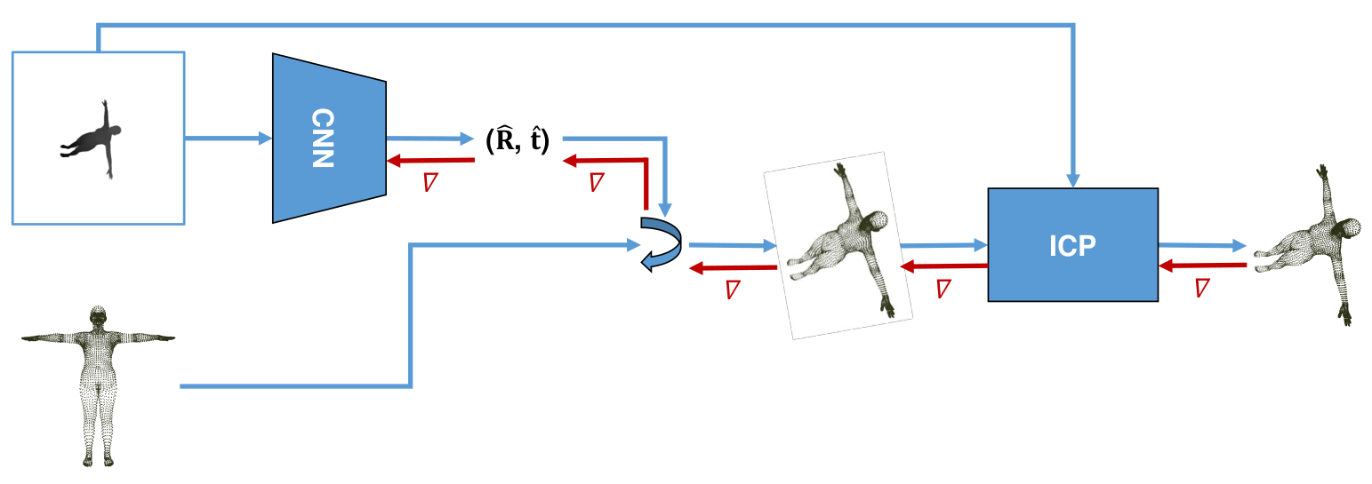
In a first experiment, we applied our point cloud reconstruction approach to a toy dataset that we created ourselves by rendering an SMPL body model with fixed body pose/shape parameters from randomly selected viewpoints. By rotating and translating each sample by a random amount, we then obtained pairs of point clouds that we could later try to match.
We compared our approach of neural network plus ICP to both the neural network and ICP on its own. The result is shown in the following figure, where we plotted the percentage of samples that were correctly predicted (Y-axis) based on the initial distance of the two respective point clouds (X-axis). The line styles represent different versions of “correctness” where straight lines represent an error margin of 3 cm and dashed lines an error margin of 30 cm (which is roughly 1.5% / 15% of the ~2 m model respectively).
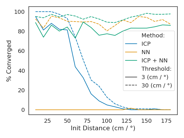
We found that the neural network (yellow) predicts poses very robustly but rarely achieves a satisfying accuracy. ICP (blue), on the other hand, can be very precise, but it only works well if the initial distances are already small. As shown, combining optimization and learning (green) achieves similar accuracy as ICP but works robustly for all samples. Thus, it performs strictly better than either of the methods alone.
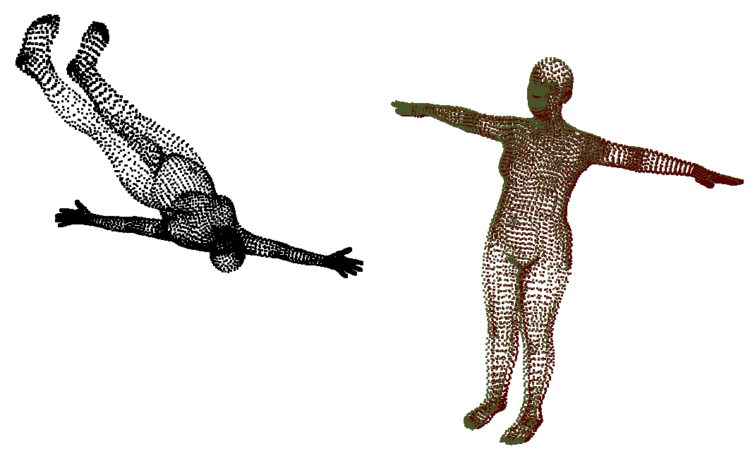
A qualitative example is shown in the teaser image, where we tried to match the black and red point clouds. As we see, they are fairly far apart and have very different rotations, which is a scenario where standard ICP would be almost guaranteed to fail. The result of transforming the black point cloud by the predicted pose of our method is shown in green, and, as we see, the fit is very accurate.
End-to-End Point Cloud Reconstruction on ModelNet40 Benchmark
Since our hybrid approach worked very well on the toy problem, we decided to apply it to the ModelNet40 dataset, which is a popular point cloud reconstruction benchmark.
In this problem setting, we always match two point clouds (not depth maps), so we decided to use the state-of-the-art learning-based method Deep Closest Point (DCP) as the neural network predicting initial poses and trained it end-to-end with our differentiable ICP.
To evaluate our proposed approach, we compared it with several point cloud registration methods based on both optimization (ICP, Go-ICP, FGR) and learning (PointNetLK, DCP). We measured the performance according to six different metrics (MAE/MSE/RMSE of rotation/translation). The results are shown below.
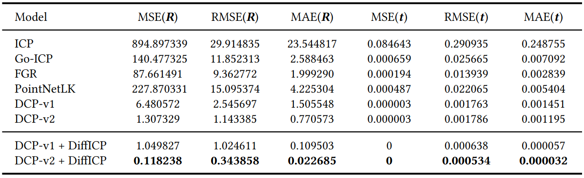
As shown, our method significantly outperforms all others and achieves the best scores reported on the dataset thus far. Most notably, combining DCP-v2 with our differentiable ICP reduced its error by over 70% across all metrics (60% for DCP-v1).
Result
We developed a fully-differentiable PyTorch implementation of ICP which can be used as a building block in ML architectures. With a combination of learning and differentiable optimization, we managed to beat state-of-the-art point cloud reconstruction methods on a popular benchmark, achieving an over 70% lower error across six metrics. However, the theoretical contributions of the project were rather small, so it was unlikely to get published (which means failure in academia).
Next Steps
We planned to further expand upon the differentiable point cloud reconstruction with the goal of ultimately developing a superior method for clothed human body reconstruction.
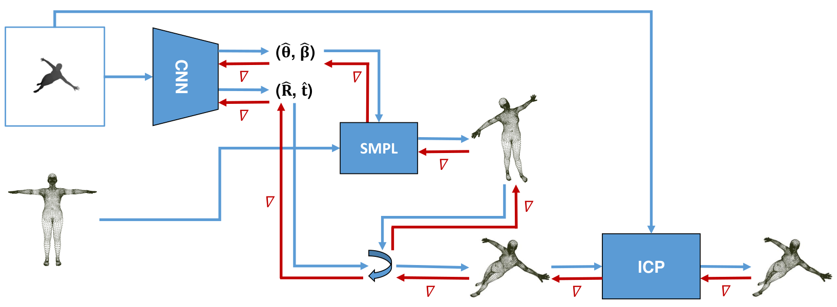
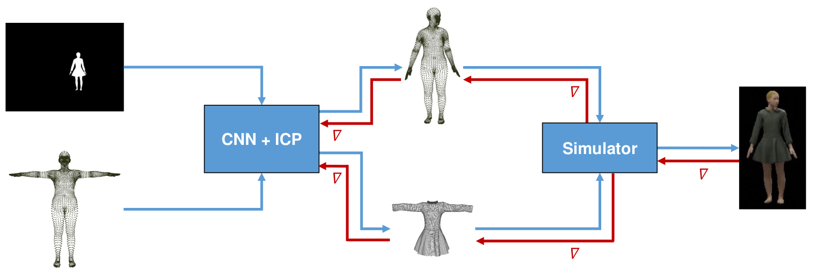
First, we wanted to not only fit the rigid pose of an object with ICP but also the non-rigid body deformations, which we wanted to model using an SMPL body model (which is fully differentiable). To do so, we planned to modify our neural network to also predict SMPL pose and shape parameters and then jointly optimize all parameters using a differentiable non-rigid ICP. This is shown below.
Afterwards, we planned to also fit clothing in a similar way by writing a fully differentiable clothing simulation based on physical properties, which would then allow us to train the whole pipeline end-to-end.
We started working on these ideas but didn’t bring any of them to completion since the project was halted after I quit my PhD.
Discussion: Does ICP necessarily need to be fully-differentiable?
Yes and no. It depends on what you want to do with it.
If you want to train a learning-based method that predicts an initial pose which should subsequently be refined with ICP, then full differentiability is needed for end-to-end training. This can be seen by considering that for fixed correspondences the ICP algorithm will always find the same optimal transformation in each step, independent of the initial rotation and translation of the two objects. Thus, if the correspondences do not provide non-zero gradients, the gradients of the entire ICP will be all zero with regard to the initial pose.
However, if we wish to train other methods that, e.g., generate the surfaces themselves instead of their 3D pose, even the gradients of an ICP with non-differentiable correspondences might still be meaningful.
Now, is it useful to backpropagate through ICP in the first place? In our application of point cloud reconstruction, it did allow us to achieve better results, but the improvement was negligible in the grand theme of things. Also, backpropagating through an iterative optimization is inherently unstable as the magnitude of gradients can vary strongly, so we can only run for a fixed predefined number of steps during training, which then deviates from the test-time behavior again. Furthermore, even with a fixed number of steps, the success of learning is still highly dependent on specific hyperparameter choices, so the model training overall becomes significantly more complicated and also much slower.
In summary, yes, it can be useful, but it is most likely not worth the effort.
Takeaways
-
Many graphics problems can be solved by either learning or optimization. Learning is usually faster and more robust, whereas optimization is more accurate. Combining the two approaches is both robust and accurate and can thereby achieve better results than any of the individual methods.
-
When implementing an algorithm, tailor it to your language and underlying hardware. In the ICP example, people used to build sophisticated algorithms and data structures for finding approximate nearest neighbors in point clouds, but with modern GPUs, it is much faster to simply compute the exact nearest neighbors with a few matrix multiplications.
-
End-to-end training sounds compelling, but it’s mostly just a buzzword that might help you sell your paper. What is rarely mentioned is how much slower and more complex the training can become, which can outweigh the benefits. In the end, there are probably more effective and more meaningful ways of improving upon existing work than simply making operations differentiable.