An Analysis of ICP Variants

Over the years, various ICP modifications have been proposed. Now, which one should you use? Well, it depends on your use case. As a researcher, your goal might be to get the highest accuracy score out of it. Or perhaps you’re making a real-time demo and speed is your main concern. Then again, you might be a developer building the next unicorn app and want to achieve good performance under varying conditions. As we see, the requirements for ICP applications can vary hugely.

In the following, we will analyze and compare the most common ICP variants and find out which combination of design choices is best for each of the use cases outlined before.

Sampling

If you’re dealing with giant point clouds, as can for instance be the case when trying to scan whole buildings, it might make sense to only use a subset of the available points for your ICP. For how to select those points, various options exist, most of which are based on random sampling. However, the tradeoffs are often minor, so most of the time you can ignore all the fancy sampling strategies and just stick to plain old uniform random sampling.

How densely should you sample? That depends on your project goals again. Generally, as with all data-driven methods, the more data the better, but also the more data the slower. However, there are diminishing returns. Often you can be able to recognize whether point clouds are unnecessarily dense, too sparse, or just right, simply by looking at them in MeshLab or similar.

My personal recommendation: Ignore sampling at first and just build your ICP and try it on your use case. Then, if you want it to be faster, reduce the number of points as needed (and/or adjust other options covered in the following sections).

Correspondence Search

Standard ICP correspondences are found by searching the nearest neighbor of each source point within the target point cloud. However, many variations have been proposed, most notably:

If surface normals are available, normal shooting can be used where we shoot a ray from the source point into the direction of it’s surface normal and search for the intersection with the target surface,
For depthmap inputs, projective correspondences can be found by projecting each source point onto the target depthmap.

The main point to understand here is that both of those methods are intended to be approximations of the full nearest neighbor search. Thus, as one would expect, normal shooting and projective correspondences are faster but less accurate/robust.

Also, a very important detail: both of those approximate methods are surface-based, so they need to be combined with a surface-based error metric like point-to-plane or symmetric ICP (see below), i.e., do not use normal shooting or projective correspondences with point-to-point.

Correspondence Weighting/Rejection

Optionally, we can then assign weights (for the later optimization) to each correspondence and/or discard (reject) correspondences that we deem incorrect. Again, there have been several methods proposed for both, but the most commonly used techniques are:

Linear weighting based on point-to-point distance
Weighting based on the similarity of surface normals (dot product)
Rejection of correspondences where the point-to-point distance is higher than a predefined threshold
Rejection of correspondences where the similarity of surface normals (dot product) is less than a predefined threshold

The main takeaways here are:

Rejection significantly increases accuracy and speed but reduces robustness
Weighting increases accuracy but slightly reduces robustness and speed
Rejection and weighting complement each other: weighting allows us to choose a less tight rejection threshold, thereby achieving a similar accuracy with improved robustness

Note that we can also incorporate rejection into any of the correspondence finding methods by restricting our search to only those target points that match other criteria, like a similar surface normal direction. To find a correspondence, we would then perform an additional iterative search for each point. This is sometimes called Closest Compatible Points. However, in practice, the performance of such methods is usually not much better than separate matching and rejection steps but has a significantly longer run time due to the iterative searches. For this reason, it is usually not worth the effort.

Error Metrics & Minimization

Before we talk about minimization, let’s recap what error metrics are there. In almost all applications that you will encounter, either the point-to-point or the point-to-plane distances are used. Those are by far the most popular. However, I want to highlight another metric here, the recently published Symmetric ICP, which is basically a strictly better version of point-to-plane.

To minimize these metrics, we have three options:

Direct calculation of the analytical solution: This option is fast and as accurate as it gets. The only problem is that this is only possible for the point-to-point metric (via Procrustes analysis).
Approximation via linearization: Here we assume that the two objects are already well aligned, i.e., that the rotation between them is small, which then allows us to find a solution by solving a linear system of equations. Out of all the methods, linearization is the fastest, but due to its assumption of small angles, robustness and accuracy suffer.
Approximation via optimization: Lastly, we can optimize for any given metric using our favourite optimization methods like LM. Unlike the other two methods, optimization is iterative, and, therefore, significantly slower. However, unlike linearization, it is fairly accurate.

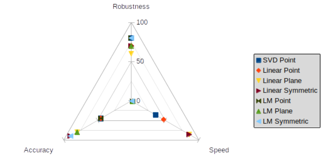
In the teaser image, a full comparison of all metric-minimization combinations is shown, for which I quantitatively evaluated all versions on a point cloud reconstruction task under otherwise similar conditions and assigned them a score between 0 and 100 on three axes:

Accuracy is measured as the fraction of easy (low initial distance) samples converging below a given error threshold (~1.5 of the model size),
Robustness is measured as the maximum rotation (in degree) between point clouds where the respective ICP variant can still converge at least 50% of the time to an accurate solution,
Speed is the algorithm’s run time, measured in samples per second (in my PyTorch implementation; Note that this is not the same as iteration speed, since my definition also takes the number of iterations until convergence into account, which is why, e.g., point-to-point tends to be ranked lower).

To summarize the plot, we found that:

For point-to-point, the analytic solution via Procrustes is best overall,
Symmetric ICP is strictly better than point-to-plane,
Accuracy depends mostly on the error metric, with Symmetric ICP > point-to-plane » point-to-point,
Linearization is less robust than the other two minimization methods and
Point-to-plane is less robust than the other two metrics (for unknown reasons),
linearization is fastest and optimization is the slowest by far and
point-to-point is slower than the other metrics (because it needs more iterations to converge)

Which ICP variant is best?

Let’s now summarize our findings outlined above and answer the question we posed in the beginning: which ICP variant should you use?

The fastest ICP

If speed is the main concern, use:

Uniform random sampling of as few points as possible (needs to be tuned manually),
Approximate correspondences, e.g., via projection,
Correspondence rejection based on both distance and normals with as tight thresholds as possible,
Point-to-plane or Symmetric ICP minimized via the linearization method.

The most accurate ICP

To get the most accurate ICP fit, use:

No sampling,
Full nearest neighbor correspondences,
A combination of both correspondence weighting and rejection for both distances and normals, with carefully tuned rejection thresholds,
Symmetric ICP (alternatively point-to-plane) minimized via LM optimization.

The most robust ICP

Finally, if your ICP needs to work even for poorly aligned inputs, consider:

Full nearest neighbor correspondences,
No correspondence weighting/rejection,
Either point-to-point minimized via Procrustes or symmetric ICP minimized via LM optimization.

The best ICP

So, what if all of those aspects are important to you? What’s the best version overall? If I had to pick one configuration to use everywhere, I would choose:

Uniform random sampling of a moderate amount of points (should be tuned manually for given data)
Full nearest neighbor correspondences,
A combination of both correspondence weighting and rejection for both distances and normals with tight rejection thresholds,
Symmetric ICP (alternatively point-to-plane) minimized via linearization.